Memory of the Earth – lakes as landscape archives
In the previous blog post, we learned about the glacial cirque lakes in the Black Forest and the Vosges and their history. In this blog post, we get to know these places as landscape archives.
Landscapes can preserve information on their past in geological, biological and sediment traces and can therefore be seen as archives for Earth history.
Pollen diagrams
To give an example, plant pollen can be seen as probes from the past. When you do landscape photography in early summer, you might experience the situation like shown in the following figure.
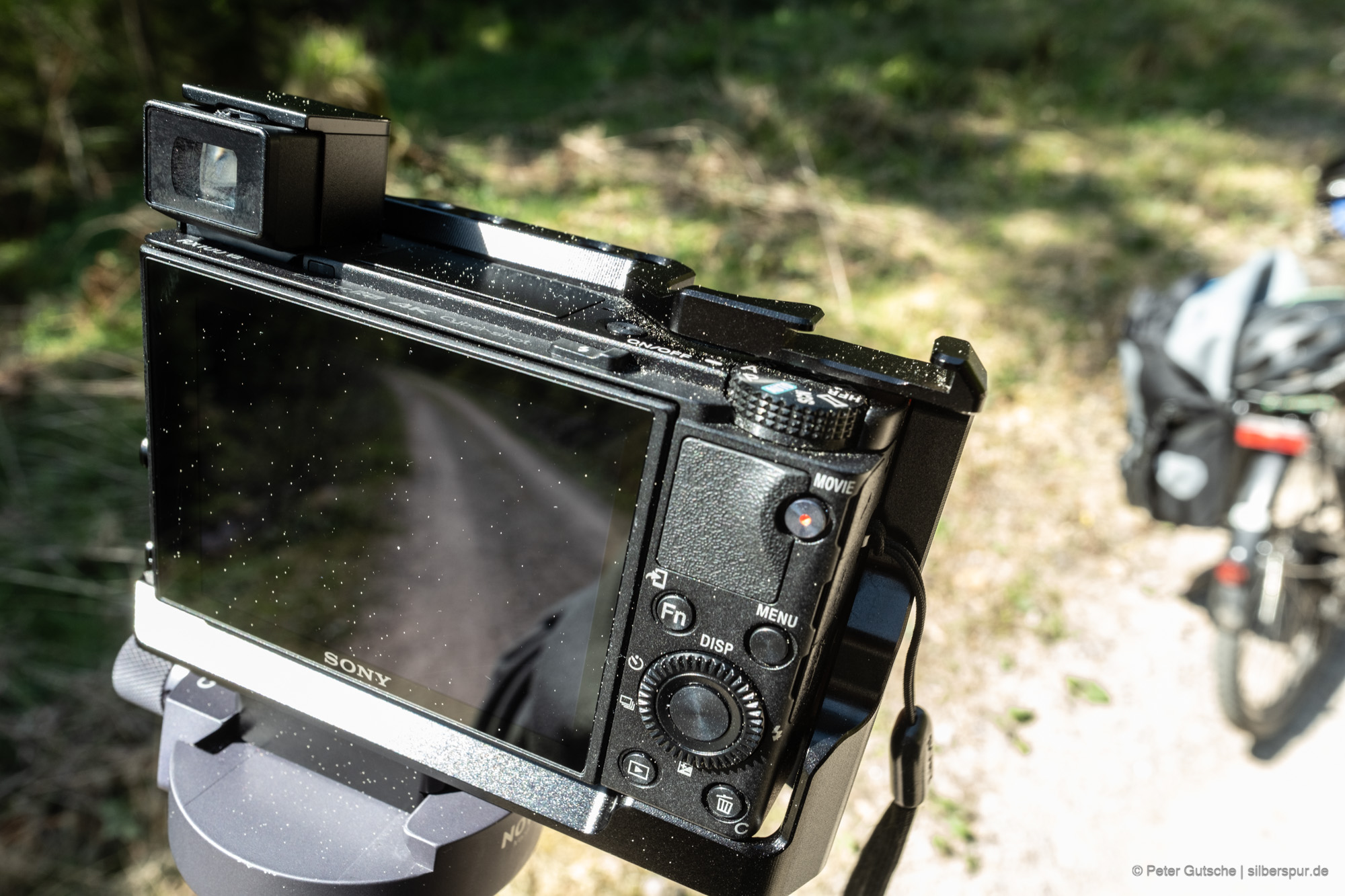
The little spots are plant pollen that settle down on objects like cameras. Due to their low weight, pollen can be carried in the air for a long time and then sink down to the surface of the Earth and get deposited together with other material. Still waters are ideal collection ponds. The tiny particles fall down to the water surface and sink slowly down to the ground. In still lakes and peat bogs, this process can happen slowly without any disturbance, so that year after year a new layer of sediment can form on the ground. The deeper the layer, the older the material is that it holds. That means, a sediment layer in a certain depth contains material that has sunk down to the lake at a certain time in Earth's past.
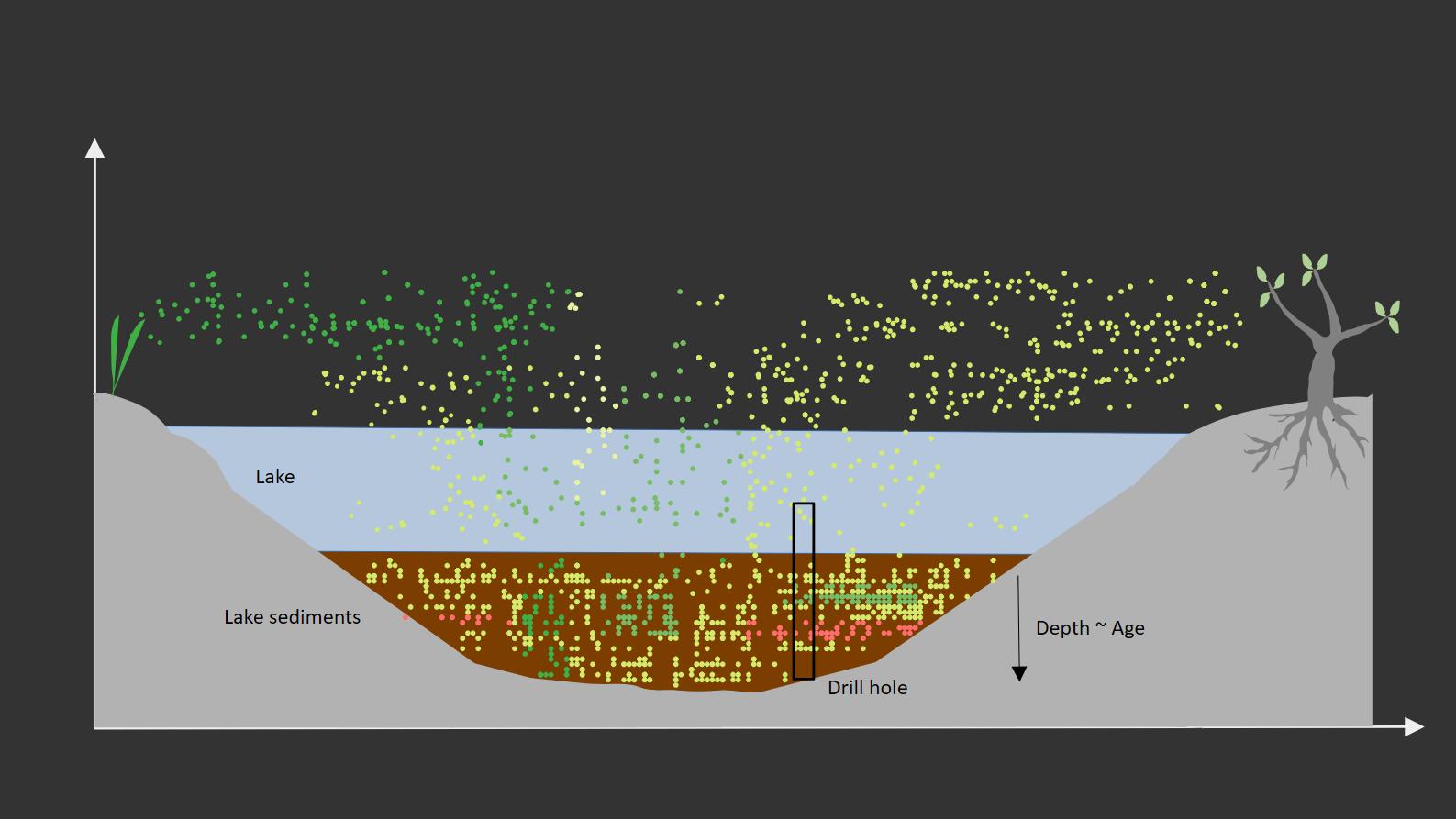
Analysis of pollen (palynology) makes use of the fact that pollen are very resistant and can be preserved over large periods of time. The composition of pollen in a sediment layer allows us to conclude which vegetation dominated in the vicinity of the lake at the time when the pollen sank to the lake bottom. As vegetation strongly depends on climatic conditions, the pollen composition can be seen as a climate proxy. (Learn more)
One level of complexity arises from the fact that pollen – again, due to their low weight – can be transported over large distances by winds. Therefore, the composition of pollen in a sediment layer (the pollen spectrum) does not necessarily represent the local vegetation in the vicinity of the lake. However, there is a rule of thumb: The smaller the area of the collection point (for example, the water surface area of the lake), the more the pollen spectrum represents the local vegetation. (Learn more)
The 8 tarns that still exist in the northern Black Forest (see https://www.silberspur.de/blogs/read/114), therefore, are ideal landscape archives that bear good conditions to do pollen analysis.
The archaeologist Manfred Rösch and his team have performed palynological studies at Herrenwieser See. The publication contains further details about the method. (Learn more)
We look into some of their pollen diagrams in a minute.
Dating methods
It sounds obvious: The deeper a sediment layer, the older it is. How can we determine quantitatively the age of a layer? In the Earh sciences different dating methods are used. We discuss two of them.
Dendrochronology
This method allows you to determine the age of material up to the age of several millennia. It is based on the analysis of tree rings. (Learn more)
The width of tree rings depends on environmental factors such as temperature and moisture in the growing season. Due to this, tree rings can also be used as climate proxies.
Besides this, they can also be used as a dating method. As the width of a tree ring depends on the environmental conditions in the growing season, each tree in a certain area forms a pattern of tree rings that is determined by the sequence of climate conditions in the specific area. Trees growing up in the same area in the same time period will, therefore, form a similar tree ring pattern – because they experience the same environmental conditions. A tree ring pattern – the specific sequence of rings with different widths – is therefore typical for a region and time period – like a fingerprint.
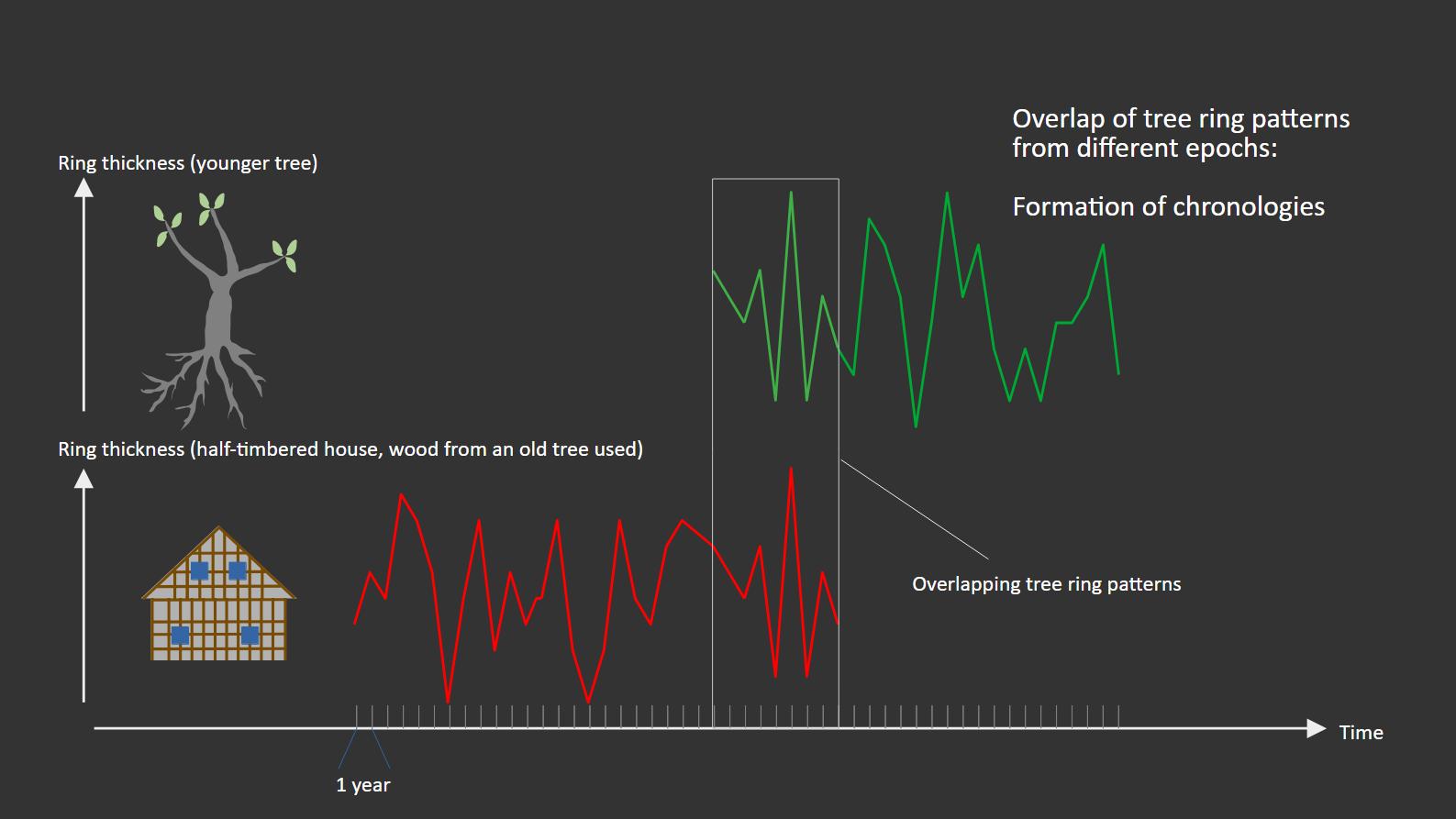
By examining tree rings with overlapping tree ring patterns – that means, from trees that lived in different growing seasons which partly overlap – it is possible to build up chronologies that reach back many millennia into the past. (Learn more)
Dendrochronology allows you to precisely date wood samples, for example, from archaeological sites.
Radiocarbon method
Radioactive materials can be used to develop dating techniques as well. (Learn more)
A well-established method to determine the age of organic material up to approximately 60 000 years into the past is the radiocarbon method. It is based on the radioactive decay of the carbon isotope ${}^{14}\mathrm{C}$. Isotopes are variants of a chemical element that differ in the weight of the atomic nucleus but have (to a large extent) the same chemical properties. The atomic nucleus is composed of protons (positively charged) and neutrons (electrically neutral). The number of protons determines the chemical element (for example, if we talk about carbon or nitrogen).
Isotopes of the same chemical element have, strictly speaking, the same number of protons but a different number of neutrons. To indicate isotopes, there is the convention to write the total number of nucleons (protons + neutrons) as a superscript to the left of the element symbol, for example, ${}^{12}\mathrm{C}$ or ${}^{14}\mathrm{C}$ for different carbon isotopes. (Learn more)
Most isotopes that occur in nature are stable. Some isotopes, however, are unstable (radioactive). Their nuclei tend to decay and, in that way, transform into another isotope. (Learn more)
The most common carbon isotope occurring in nature is the stable isotope ${}^{12}\mathrm{C}$ (6 protons + 6 neutrons). The isotope (${}^{14}\mathrm{C}$), however, has 6 protons and 8 neutrons and is unstable. In nature, it occurs only in tiny traces, with an abundance of about $1.25 \cdot 10^{-10}$ % (of the total carbon).
${}^{14}\mathrm{C}$ is continually created in the upper atmosphere through the reaction of nitrogen atoms (${}^{14}\mathrm{N}$) with neutrons that originate in cosmic radiation. (Learn more)
The newly formed ${}^{14}\mathrm{C}$ chemically combines with oxygen to form the gas carbon dioxide – in the same way as the more abundant ${}^{12}\mathrm{C}$. ${}^{14}\mathrm{C}$, as mentioned, is radioactive and decays with a half-life of about 5700 years. This means that, considering a large number of such atomic nuclei, after this time half of them will have decayed and transformed back into nitrogen nuclei ${}^{14}\mathrm{N}$. (Learn more)
As through the exposure of the upper atmosphere to cosmic radion constantly new ${}^{14}\mathrm{C}$ nuclei are produced, however, these decay with a certain rate, the system moves into a state of dynamic equilibrium (also referred to as flow equilibrium) with a constant concentration of ${}^{14}\mathrm{C}$.
One can illustrate a flow equilibrium using the analogy of a bathtub:
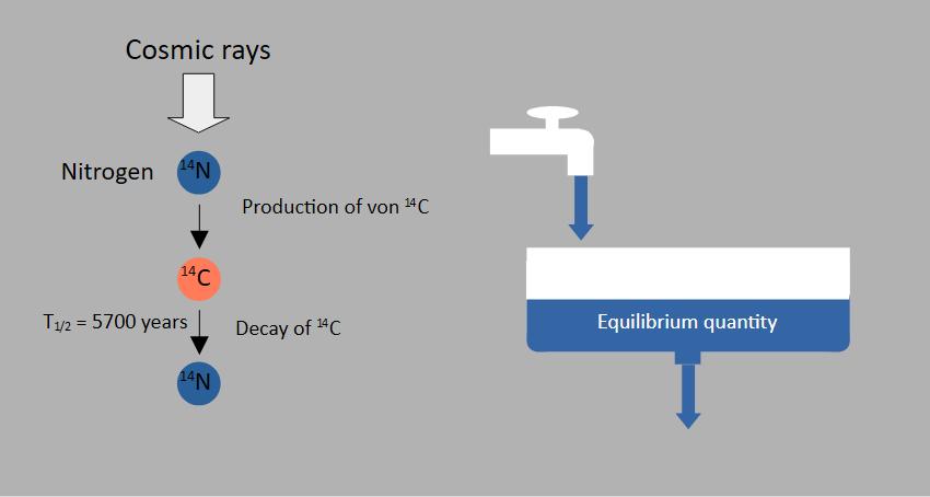
Imagine a bathtub where water is filled in from above at a constant rate and that loses water through a hole. The outflow rate depends on the water pressure, that means, on the water level. The water rises until the pressure is high enough so that the outflow rate equals the inflow rate. Then, the system is in equilibrium.
Analogous to this, in the upper atmosphere a constant concentration of ${}^{14}\mathrm{C}$ is established when the production rate (by cosmic radiation) equals the decay rate (a property of the isotope).
Some ${}^{14}\mathrm{C}$ atoms built in the atmosphere chemically combine with oxygen to form carbon dioxide($\mathrm{CO_2}$) – in the same way like the more abundant ${}^{12}\mathrm{C}$ do. Therefore, the carbon dioxide in the air contains a (tiny) amount of molecules that have a ${}^{14}\mathrm{C}$ atom instead of a ${}^{12}\mathrm{C}$ atom.
When doing photosynthesis, plants absorb carbon dioxide from the air – that means, to a certain extend also carbon dioxide with the rare ${}^{14}\mathrm{C}$. In this process, plants use light energy from the sun to form organic glucose from carbon dioxide and water, while simultaneously releasing oxygen. During the lifetime of a plant – as long as the plant performs photosynthesis and is in exchange with the carbon reservoir of the atmosphere – the organic material of the plant holds a certain concentration of ${}^{14}\mathrm{C}$ that is equal to the ${}^{14}\mathrm{C}$ concentration in the atmosphere.
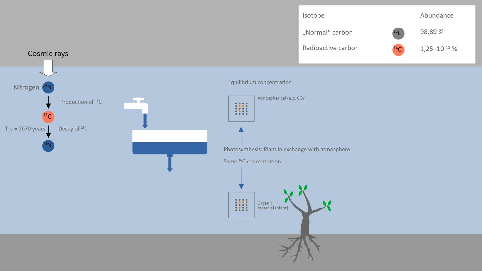
As soon as a plant dies, as the process of photosynthesis ends, it becomes decoupled from the carbon reservoir of the atmosphere. From that moment on, the radioactive 'clock' begins to 'tick': Due to radioactive decay, the amount of ${}^{14}\mathrm{C}$ decreases continually without new such isotopes coming in. When you examine the amount of ${}^{14}\mathrm{C}$ in an old piece of wood that is installed, for example, in an old half-timbered house, you can conclude the age of the house. More precisely, you can conclude the time that has passed since the tree from which the wood comes was cut down and has, therefore, stopped being in exchange with the atmospheric carbon reservoir by doing photosynthesis. (Learn more)
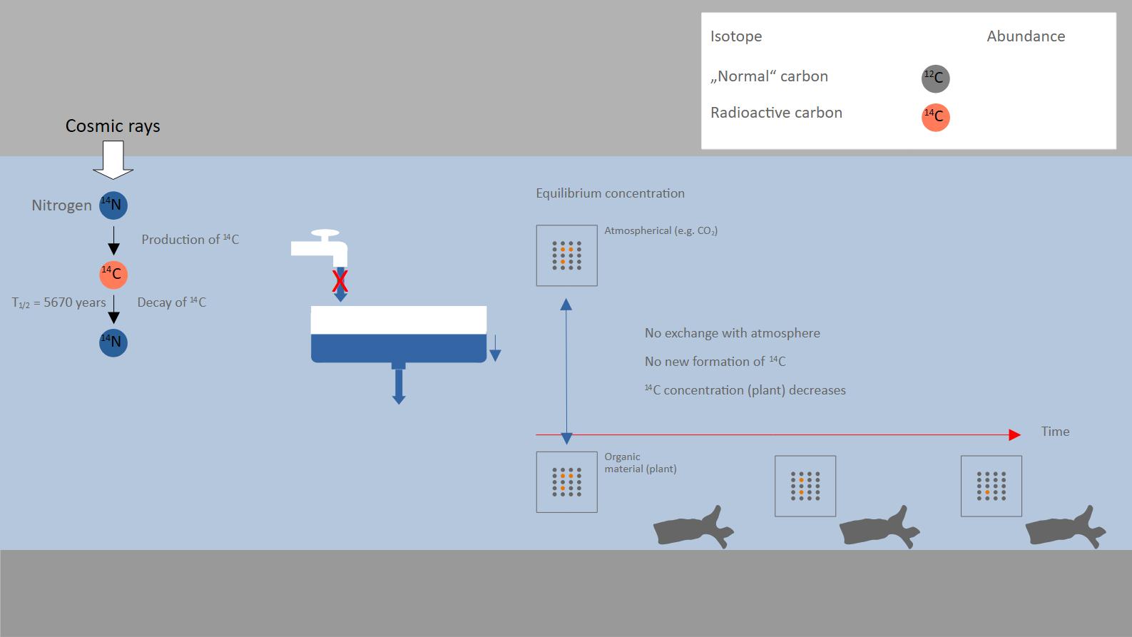
As a summary, as soon as the plant system is isolated from the carbon reservoir of the atmosphere, where constantly new ${}^{14}\mathrm{C}$ is produced, the radionuclides in the plant act like a 'clock'. It is easy to modify the analogy with the bathtub used to illustrate the flow equilibrium – where the inflow is stopped at a certain time (when the plant dies) – to the analogy of an hourglass. As long as the plant lives, new sand is filled into the upper compartment of the hourglass at a constant rate. At a certain moment (when the plant dies), the upper compartment is closed, and then the sand runs at a constant rate through the hole in the middle without new sand coming in from above. (Learn more)
The radiocarbon method was used, for example, to determine the age of the glacier mummy 'Ötzi', who was found in the Ötztal Alps (on the border between Italy and Austria) in 1991. (Learn more)
Without going further into the details, it needs to be mentioned that reality is a bit more complicated. Indeed, the atmospheric concentration of ${}^{14}\mathrm{C}$ is, seen over longer periods of time, not stable. Changes in sloar activity and cosmic radiation can have an influence on the production rate of ${}^{14}\mathrm{C}$ in the upper atmosphere. A reduced solar activity leads to an increased flux of cosmic radiation and that way to a higher production rate of ${}^{14}\mathrm{C}$. (Learn more)
There are other factors as well that have a direct influence on the concentration of this isotope in the atmosphere. These include volcanic eruptions and anthropogenic inputs of carbon dioxide into the atmosphere. Accordingly, measurements of the remaining ${}^{14}\mathrm{C}$ concentration of a sample under investigation must be calibrated using other dating methods. (Learn more)
Pollen diagrams from sediments of the tarns in the northern Black Forest
Now we understand how we can transkate the depth of a sediment layer into its age.
We now inspect a pollen diagramm that was derived from the sediments of the Huzenbacher See in the northern Black Forest. With kind permission from Prof. Dr. Manfred Rösch of Heidelberg University, Institute of Prehistory and Early History and Near Eastern Archaeology.
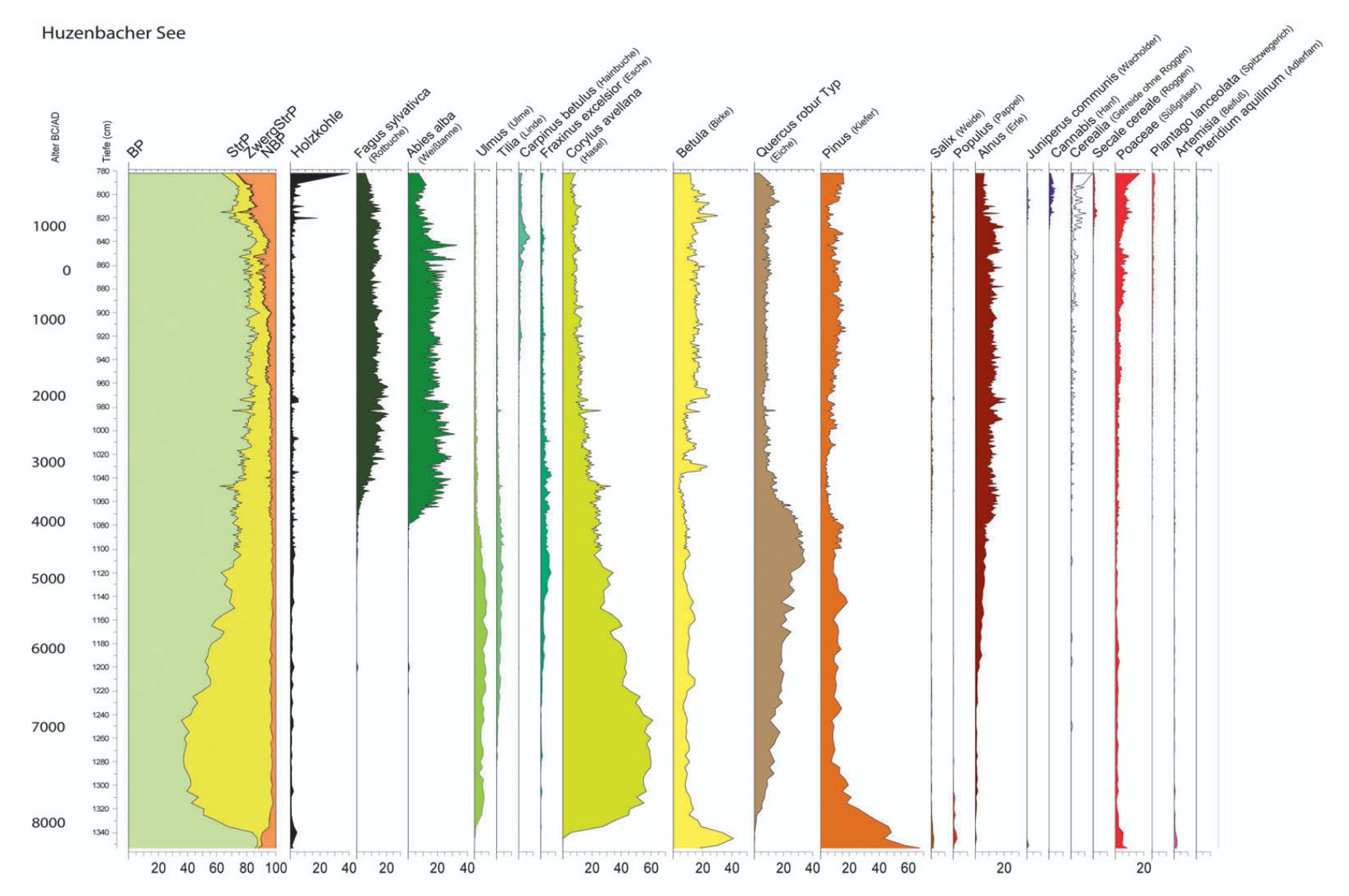
The vertical axis represents the depth of the sediment sample, which corresponds to time (as derived by radiocarbon dating), with the deepest and oldest deposits at the bottom and the most shallow or recent deposits at the top. The years BC (before Christ) and AD (after Christ) are already indicated there.
On the horizontal axis, from left to right, individual pollen diagrams for different plant species are shown. The horizontal axis of each such diagram plots the percentage of a given pollen type present in the sample. Each plant species is represented by its own separate curve. By convention, similar patterns are grouped together on the diagram, with arboreal types (trees) shown first, followed in turn by shrubs and herbs. At the far left, pollen types are summarized into two groups: non-tree pollen (Nicht-Baumpollen, NBP) and tree pollen (Baumpollen, BP). (Learn more)
In simple terms, can we derive the following conclusions from this diagram about the development of vegetation in the Huzenbacher See area since the end of the last glaciation:
- In the 9th millennium BC, the area was already completely forested – predominantly with pines and birches.
- From the 8th millennium onwards, these trees were pushed back by hazel. In the following centuries, elm and oak trees migrated into the region.
- During the 6th millennium BC, the overall appearance of the landscape was dominated by a mixed oak forest that also contained linden and ash trees. The proportion of hazel shrank continuously.
- Only from the 4th millennium BC onwards do the pollen diagrams show significantly increasing signals from silver fir and European beech. These trees dominated the landscape in the following millennia.
This means that at the beginning of the Holocene, the Black Forest did not yet have the appearance that gave this landscape the name Silva Nigra in historic times. (Learn more)
Gradually, the landscapes north of the Alps were populated with different forest communities. Until about 6000 years ago, the Black Forest was a deciduous forest with oak, linden, elm, ash, maple, hazel and birch – as suggested by palynological studies. Only from that time on, fir and beech trees began to populate and to partly push aside the woods that have dominated the landscape until then. (Learn more)
We conclude that landscapes are not as stable as they seem at first glance. Instead, they show a dynamic history. When you hike in the northern Black Forest nowadays, you find yourself in a landscape dominated by extensive dark coniferous forests.
The following figure shows a synopical representation that compares pollen diagramms from the 8 tarns and two peat bogs in the northern Black Forest. In this representation, the pollen spectra are not broken down into individual plant species. Instead of this, it is only differentiated (for each location) between non-arboreal pollen (Nicht-Baumpollen, NBP) and shrub pollen (Strauchpollen, StrP – mainly considering hazel). This coarser grid has the effect of a filter that makes visible specific overall developments. With kind permission from Prof. Dr. Manfred Rösch of Heidelberg University, Institute of Prehistory and Early History and Near Eastern Archaeology.
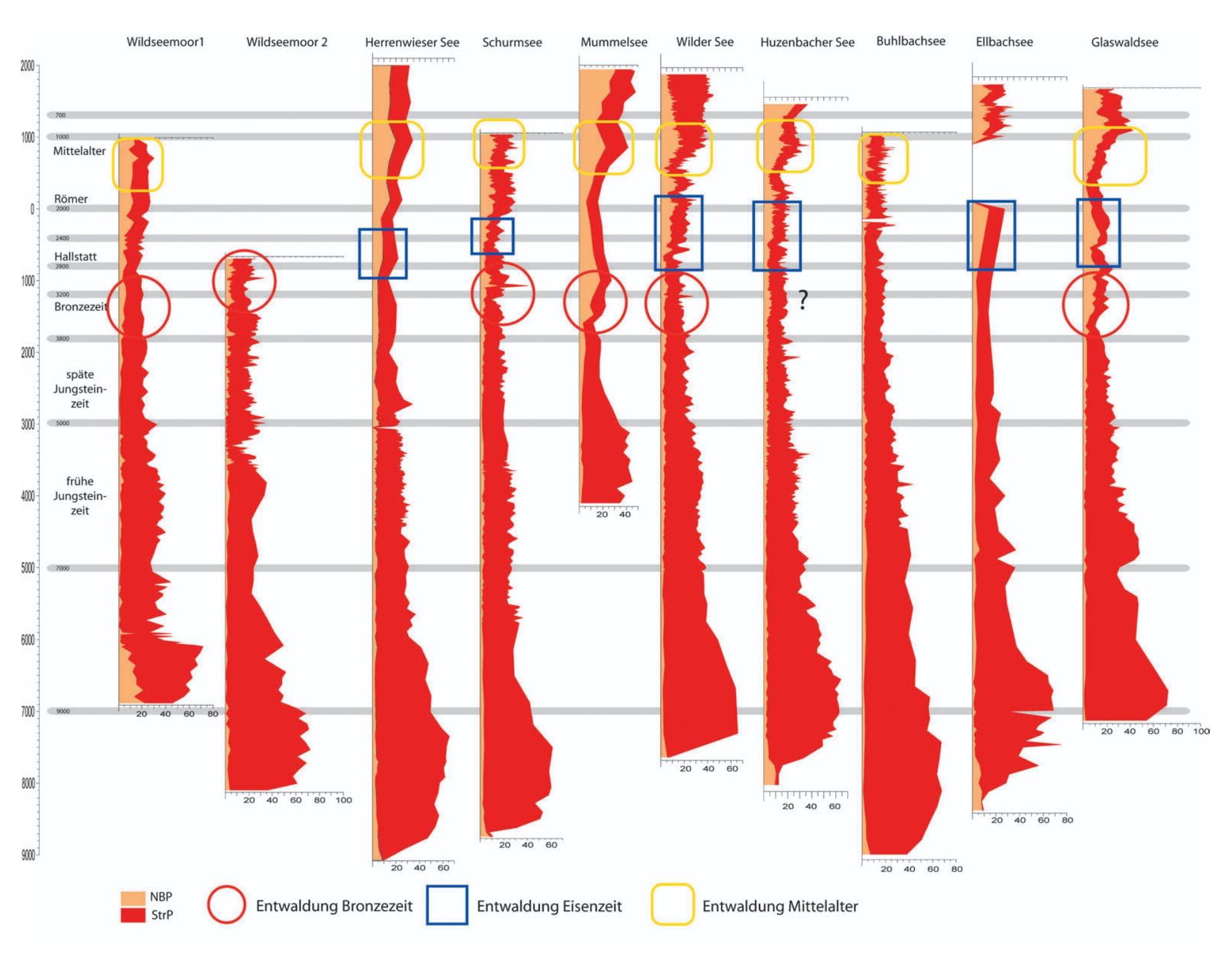
In this representation, as indicated in the figure by circles and rectangles, periods with an increased signal of NBP can be interpreted as phases with deforestation caused by humans. Therefore, these pollen spectra can be interpreted in such a way that there was already human influence in the vicinity of the study locations in the Bronze Age (about 3800 and 3000 years ago; red circles), in the Iron Age (between 2800 and 2000 years ago; blue rectangles), and then, very clearly indicated, starting from the early medieval time (yellow rectangles).
The botanist and geographer Burkhard Frenzel (1928 – 2010) points out that the Black Forest was populated very early and that pastoral economy was practiced even in the most remote locations, which implied deforestation. (Learn more)
Assarting led to the formation of peat bogs that characterize the landscape until today. These peat bogs are also called Missenmoore in German. (Learn more)
The time scale of the presented palynological studies leads us back to the beginning of the Holocene some 11 000 years ago. (Learn more)
Human influence
We have seen that pollen spectra as derived from landscape archives allow os to derive conclusions on human influence back in the past.
In the past, the rafting of timber played an important role in the development of the landscape. In the Mummelsee episode from Grimmelshausen we referred to at the end of the first blogpost, Simplicius says:
I did inspect the lake, and found lying in it certain hewn timbers which my dad and I took to be the remains of the Württemberg raft
Maybe Grimmelshausen provides a clue that during his time, shortly after the end of the Thirty Years' War, timber rafting was already practiced in locations that were very remote at that time.
Also, the geographer Fritz Fezer notes that we still find traces of human activity at some of the tarns still in the 20th century: dam structures used to swell the water in order to transport logs into the valley with the force of the water. (Learn more)
Wood was important for shipbuilding, but also as firewood. In particular, in the 18th century, wood became rare due to demographic increase and energy-intensive industries such as glassmaking. Therefore, the rafting of timber temporarily degenerated into the overexploitation of nature, which must have changed the appearance of the landscape significantly. Later reforestation resulted in a landscape that was no longer comparable to the natural landscape of earlier times. (Learn more)
Referring to human influence and a changed relationship of humans with nature Fritz Fezer writes in 1957: (Learn more)
Humans also changed their relationship with the lakes. Still in the 17th century, the beautiful Ellbachsee was drained in order to gain a few ares of poor-quality meadow, and the Wildsee was used as a swell pond for timber rafting, in the same way as the Buhlbachsee. Likely, the dam structures of the Huzenbacher See and the Glaswaldsee are from these times. Only as of this century have humans begun to change their point of view, moving away from seeing the lakes only from an economic perspective; at the Wildsee, this point of view was completely abandoned. It is also planned to dam the Buhlbach to attract tourists. If slowly refilled, the Ellbachsee could also be restored without damaging the flora. This prototype of a tarn with its powerful beauty absolutely deserves nature protection.“
In order to understand what an isotope is, let's take a short look at the atomic structure of matter. Atoms of the same 'sort' belong to the same chemical element, for example, carbon, sulphur, oxygen or nitrogen. An element has specific material properties (for example, the melting point) and chemical properties (the ability to enter into a chemical compound with another element). On an atomic scale, the chemical properties are bonding properties. Atoms can connect with other atoms (of the same or different element) and, that way, form larger bodies: molecules.
Molecules have completely different properties than their basic products. Therefore: Although only 94 elements exist in nature, the world contains many more different substances. For example: Two oxygen atoms can connect with one carbon atom to form a carbon dioxide molecule. At room temperature, oxygen is a colorless gas that humans need to breathe, and carbon is a solid substance. Carbon dioxide, however, at room temperature is gaseous.
Atoms are composed of a compact nucleus (that contains positively charged protons and electrically neutral neutrons) and a shell that contains the (negatively charged) electrons. Why such a structure is stable can only be understood when this system is treated in terms of quantum mechanics (which is outside the scope of this article).
The properties of the electronic shell determine the bonding properties of the atom. Therefore, the chemical element is determined by the number of electrons. This number equals the number of protons in the nucleus – otherwise, the atom wouldn't be electrically neutral. An atom of the element carbon has 6 protons (in the nucleus) and 6 electrons (in the shell). An element can have different 'variants' that differ in the number of neutrons. These variants are referred to as isotopes.
The word isotope is derived from Greek: isos means equal and topos means location. Isotopes are 'at the same location' within the periodic table of elements. Different isotopes of the same element differ in the structure of the atomic nucleus (they have a slightly different weight), but behave chemically largely the same.
The most abundant carbon isotope contains 6 protons and 6 neutrons, and has in total 12 nucleons. Therefore it is indicated by the following notation ${}^{12}\mathrm{C}$. To a small amount, in nature there is also the isotope ${}^{13}\mathrm{C}$, which has 7 instead of 6 neutrons (in total, 13 nucleons). Chemically, it behaves largely identically to ${}^{12}\mathrm{C}$, meaning it connects in the same way with oxygen to form carbon dioxide. The restrictive modifier 'largely' is added because different isotopes of the same element slightly differ in their weight (due to the different numbers of neutrons), by which certain chemical and physical processes go along with isotope fractionation. That means, considering chemical processes: The chemical reaction is the same but might happen at a different rate – depending on the involved isotope.
Isotope fractionation can also happen with physical processes. For example, the oxygen isotope ${}^{18}\mathrm{O}$ has a slightly higher weight than the isotope ${}^{16}\mathrm{O}$. Therefore, evaporation of water molecules containing ${}^{18}\mathrm{O}$ happens at a lower rate than of water molecules that contain ${}^{16}\mathrm{O}$. This is an important fact when looking in more detail into the topic of climate proxies in a later blogpost.
Cf. (Lunine, 2013), p. 55.
The following figure shows a small section of the periodic table with the elements carbon (C), nitrogen (N), and oxygen (O).
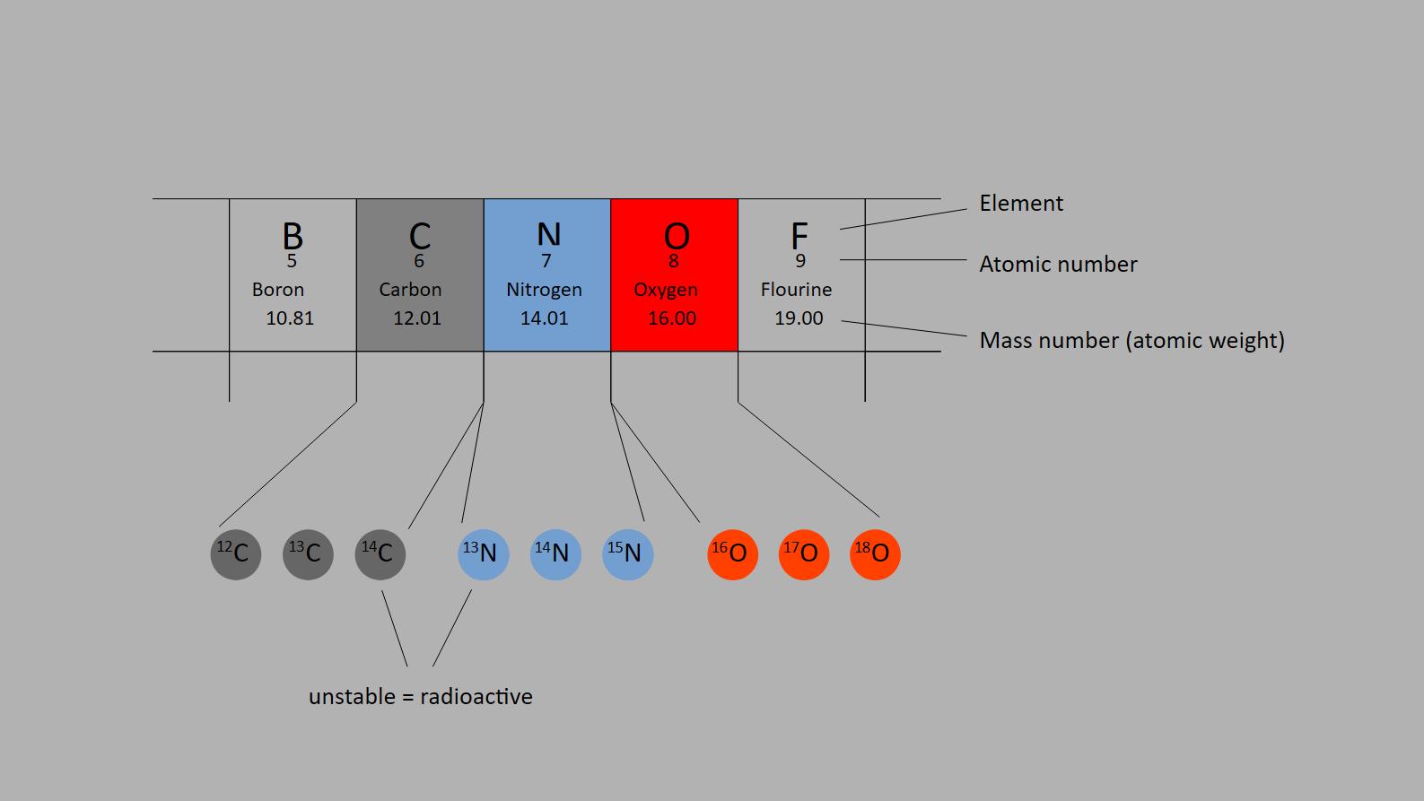
The figure also shows the isotopes of these three elements that exist in nature. The colors indicate that isotopes of the same element have the same chemical properties.
Two isotopes in the picture, ${}^{14}\mathrm{C}$ and ${}^{13}\mathrm{N}$, are unstable and decay over time into isotopes of other elements.
There are also factors that have a direct influence on the concentration of ${}^{14}\mathrm{C}$ in the atmosphere.
Volcanic eruptions can have a direct influence on the atmospheric ${}^{14}\mathrm{C}$ concentration. The carbon dioxide released during a volcanic eruption comes from geological reservoirs in the Earth's crust or the Earth's mantle and, therefore, is free of ${}^{14}\mathrm{C}$. This is due to the fact that this carbon reservoir was separated for a long time from the atmospheric carbon reservoir (where continuously new ${}^{14}\mathrm{C}$ is produced) and, therefore, has already decayed.
A similar effect has the burning of fossil resources. The carbon emitted here is also nearly free of ${}^{14}\mathrm{C}$, and carbon dioxide from fossil fuels therefore dilutes the atmospheric ${}^{14}\mathrm{C}$ concentration.
Another anthropogenic, external factor is the influence on neutron flux caused by atmospheric nuclear weapons tests. These tests significantly increased the production rate and the atmospheric ${}^{14}\mathrm{C}$ concentration, creating what is known as the „bomb pulse“. While the vast majority of atmospheric tests were conducted by the United States, the Soviet Union, and the United Kingdom in the 1950s and early 1960s—and were banned for these nations by the 1963 Partial Test Ban Treaty—France continued atmospheric testing until 1974, and China conducted its last atmospheric test on October 16, 1980. Cf. (Graven et al., 2020).
As you know, the concentration of the the gas carbon dioxide continually increases since decades – as shown by the Keeling curve.
The next figure shows the development of the atmospheric concentration of the isotope ${}^{14}\mathrm{C}$ since 1850.
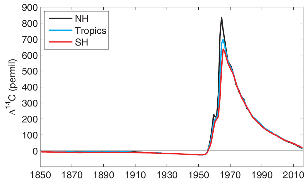
You can clearly see the peak, known as the „bomb pulse“, which was caused by above-ground nuclear tests. The most dramatic increase in ${}^{14}\mathrm{C}$ began in the 1950s as testing intensified, reaching its maximum around 1963–1965.
It is interesting to note that, apart from that peak, the ${}^{14}\mathrm{C}$ concentration has been continually decreasing for more than a century. This behavior can be explained by the fact that during this time, humans have been releasing carbon from old reservoirs into the atmosphere – namely, by burning fossil fuels.
The 'old' carbon released into the atmosphere had been decoupled from the atmospheric carbon reservoir for millions of years – because this carbon comes from plants that lived millions of years ago and were transformed into fossil fuels (coal, mineral oil) in the meantime. As discussed, this material no longer contains any measurable amount of ${}^{14}\mathrm{C}$ and, once released into the atmosphere, dilutes the atmospheric concentration of this isotope.
This is known as the ${}^{14}\mathrm{C}$ Suess effect, named after the chemist Hans Suess (1909 – 1993).
As more and more fossil carbon is released into the atmosphere, the concentration of ${}^{14}\mathrm{C}$ continually decreases, even though the absolute amount of carbon dioxide is constantly increasing.
Strictly speaking, carbon released during volcanic eruptions also originates from sources in which ${}^{14}\mathrm{C}$ has already decayed. However, volcanic eruptions are individual events that have not shown any systematic increase over the last century. For this reason, the decrease in atmospheric ${}^{14}\mathrm{C}$ concentration can only be explained by the anthropogenic release of carbon dioxide.
If you are looking for even more conclusive proof of the anthropogenic origin of increased carbon dioxide levels, you can examine the trend in atmospheric concentration of another carbon isotope, ${}^{13}\mathrm{C}$ (see also the study cited above). The concentration of this isotope has also been decreasing for many decades. This effect (the ${}^{13}\mathrm{C}$ Suess effect) can only be explained by isotope fractionation during photosynthesis – a process that slightly prefers ${}^{12}\mathrm{C}$. Consequently, fossil carbon dioxide (which ultimately originates from plants that lived millions of years ago) contains less ${}^{13}\mathrm{C}$ than atmospheric carbon dioxide. Volcanic carbon dioxide has not undergone such fractionation.
Therefore, the decrease in ${}^{13}\mathrm{C}$ is the strongest proof that the increased level of carbon dioxide in the atmosphere is caused by the burning of fossil fuels.
Returning to the radiocarbon method: All the discussed factors must be considered, and errors can be factored out using various methods. For example, dates obtained from ${}^{14}\mathrm{C}$ measurements can be calibrated using another dating method, such as dendrochronology. This is why studies using radiocarbon dating report different carbon ages: The conventional ${}^{14}\mathrm{C}$ age assumes that ${}^{14}\mathrm{C}$ production remained constant over the observation period. The calibrated carbon age is usually indicated as cal BP, where BP stands for 'Before Present'. In most cases, 'Present' refers to the year 1950, as the method was standardized in that year. Additionally, 1950 predates the systematic atmospheric nuclear testing that caused the bomb pulse.
Bibliography
- Bonani, G., Ivy, S.D., Hajdas, I., Niklaus, T.R., Suter, M., 1994. 14 C Age Determinations of Tissue, Bone and Grass Samples from the Ötztal Ice Man. Radiocarbon 36, 247–250. URL
- Bradley, R.S., 2015. Paleoclimatology: reconstructing climates of the quaternary, 3d edition. ed. Elsevier, Amsterdam.
- Fezer, F., 1957. Eiszeitliche Erscheinungen im nördlichen Schwarzwald. Selbstverlag der Bundesanstalt für Landeskunde. URL
- Graven, H., Keeling, R.F., Rogelj, J., 2020. Changes to Carbon Isotopes in Atmospheric CO2 Over the Industrial Era and Into the Future. Global Biogeochemical Cycles 34, e2019GB006170. URL
- Lang, G., 2006. Late-glacial fluctuations of timberline in the Black Forest (SW Germany): A revised approach to a climatic reconstruction. Veget Hist Archaeobot 15, 373–375. URL
- Libby, W.F., 1960. Radiocarbon dating - Nobel Lecture, December 12, 1960. URL
- Lorenz, S., Museum im Schloss (Eds.), 2001. Der Nordschwarzwald: von der Wildnis zur Wachstumsregion; die Publikation ersch. als Begleitband zum Museum im Schloss Neuenbürg. Markstein-Verl, Filderstadt.
- Lunine, J., 2013. Earth: evolution of a habitable world, 2nd ed. ed. Cambridge University Press, Cambridge. URL
- Ortlam, D., n.d. Der Ursprung der Acher (Nord-Schwarzwald) anhand historischer Recherchen sowie die glaziale Genese des Ruhesteins (Schwarzwaldhochstrasse). URL
- Reinbolz, A., Ludemann, T., 2004. Wald- und Forstgeschichte im Schwarzwald. Forstliche Versuchs- und Forschungsanstalt Baden-Württemberg, Freiburg. URL
- Rösch, M., 2012. Vegetation und Waldnutzung im Nordschwarzwald während sechs Jahrtausenden anhand von Profundalkernen aus dem Herrenwieser See. standort.wald 47, 43–67. URL
- Rösch, M., Tserendorj, G., 2011. Florengeschichtliche Beobachtungen im Nordschwarzwald (Südwestdeutschland). Hercynia N. F. 44, 53–71. URL
- Vogt, R., 2021. Flößerei auf der Acher: Ein Stück Regionalgeschichte. URL
Related Entries


